So, what exactly is a Convolutional Neural Network, or CNN? Think of it as a type of artificial intelligence designed to analyze images in a way that's surprisingly similar to how our own brains work.
A CNN doesn't just memorize an image pixel by pixel. Instead, it learns to see by identifying key features—like edges, corners, and textures—and then pieces them together to understand the bigger picture. It’s a lot like how you’d recognize a cat by its pointy ears and whiskers, not by analyzing every single dot of color.
What Are CNNs and How Do They "See" Images?
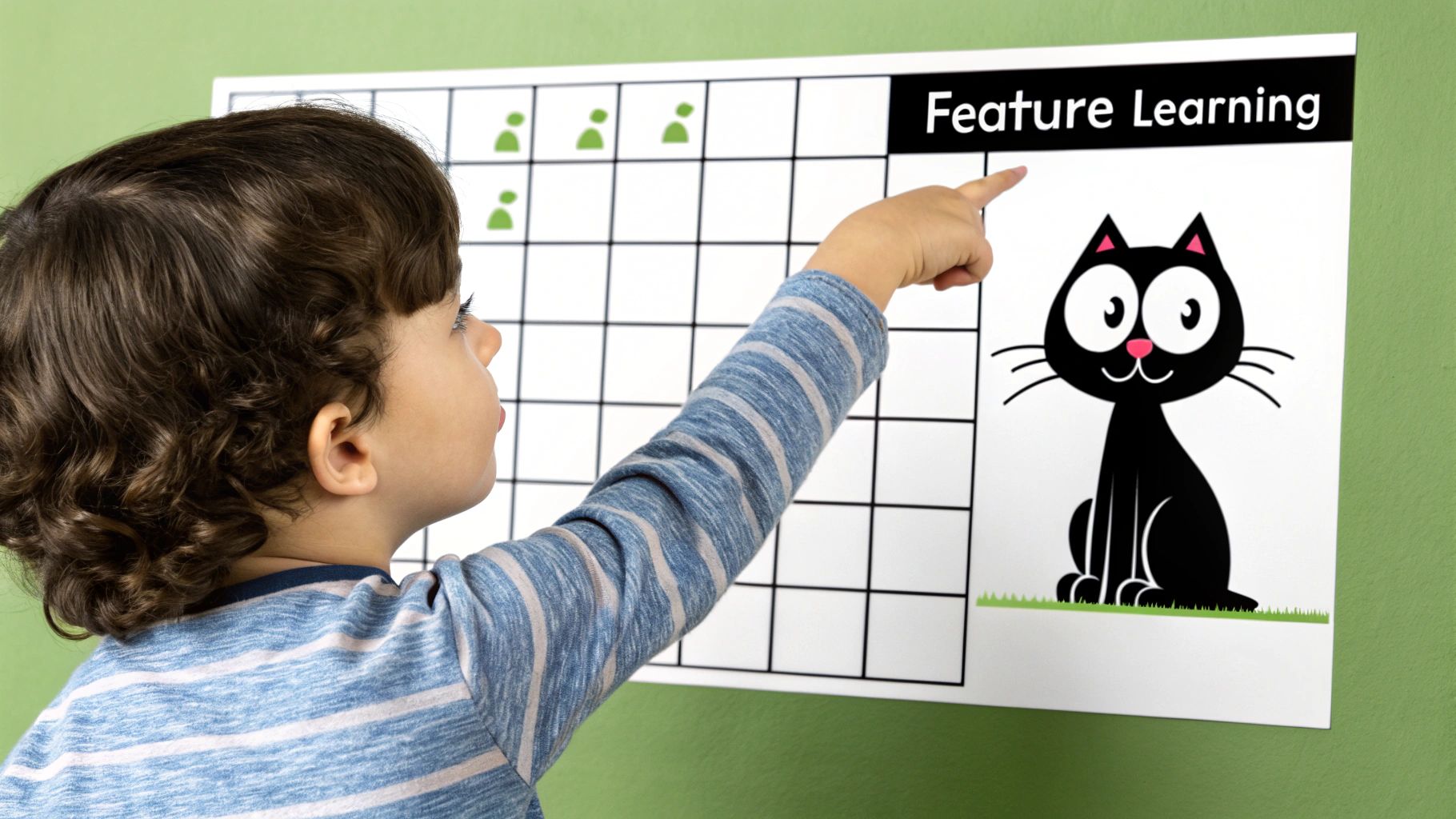
Imagine explaining what a cat looks like to a small child. You wouldn't list off the specific color values of every pixel in a photo. That would be insane. Instead, you’d point out the obvious stuff: the pointy ears, the long whiskers, the furry tail. The child quickly learns to spot this combination of features, no matter the cat's color, size, or what it's doing in the picture.
CNNs operate on this exact principle. They are the undisputed champions of image recognition because they skip the pixel-by-pixel madness and instead break down an image into a hierarchy of recognizable patterns.
Learning From Simple to Complex
A CNN starts its work by looking for the most basic building blocks of any image. In the first few layers, the network isn't looking for cats or cars; it's just trying to identify simple components like:
- Horizontal and vertical edges
- Corners and curves
- Patches of specific colors or textures
As the data flows deeper into the network, these simple features get combined into more complex patterns. For example, the network might learn that a certain curve plus a straight line often makes up an ear, or that a bunch of tiny lines clustered together represents fur.
By progressively building complexity, a CNN constructs a rich, hierarchical understanding of an image. It moves from seeing lines and colors to recognizing textures, shapes, and eventually, entire objects like faces, cars, or animals.
This feature-based strategy is a cornerstone of modern machine learning in image processing and is exactly what makes CNNs so powerful. You can dive deeper into this in our guide on machine learning in image processing.
Inspired by Biology
While CNNs feel like a recent invention, their core ideas are actually inspired by discoveries about how mammals see, going back decades. Although they exploded in popularity in the 2010s, their roots trace back much further. A prototype called the neocognitron was introduced in 1980, but its fundamental design was published by Kuniko Fukushima way back in 1979.
This groundbreaking work was directly inspired by how neurons in the visual cortex respond to things they see in their specific, localized fields of view. This bio-inspired approach is what makes CNNs so uncannily good at their job.
The Core Components Inside a CNN Model
To really get what’s going on inside a convolutional neural network, we need to pop the hood and look at the engine. A CNN isn't just one big, complicated piece of code. It's more like a sophisticated assembly line built from a series of distinct layers, each with a very specific job to do.
Think of it as a factory designed exclusively for understanding images. Raw pixels go in one end, and a confident, clear answer—like "that's a cat"—comes out the other.
This whole operation hinges on three main types of layers: the Convolutional Layer, the Pooling Layer, and the Fully Connected Layer. Each one is essential for turning a jumble of pixels into a simple, useful label.
The Convolutional Layer: The Feature Inspector
The first and most critical stop on our image assembly line is the Convolutional Layer. This is where the network really "sees." Its main job is to find important features in the image. In the very first layers, these features are super basic, like simple edges, corners, curves, or splotches of color.
So, how does it spot them? The layer uses a set of learnable filters, which are also known as kernels. You can think of a filter as a tiny, specialized magnifying glass trained to spot just one specific pattern, like a vertical line.
Here’s a step-by-step example of how one filter works:
- Define a Filter: Imagine a simple 3x3 filter designed to find vertical edges. It might look like a grid with
[1, 0, -1]in each row. - Slide Over Image: The filter is placed at the top-left corner of the image.
- Calculate: It multiplies its values with the pixel values it's covering and sums them up. A high positive value means it found a light-to-dark vertical edge. A high negative value means dark-to-light. A value near zero means no edge.
- Repeat: The filter slides one pixel to the right and repeats the calculation. It does this for the entire image, creating a new grid called a feature map. This map highlights exactly where in the image the vertical edges were found.
A single convolutional layer might have dozens or even hundreds of these filters, each one hunting for a different primitive feature. This is how a CNN starts building its understanding of an image—from the ground up, one tiny visual clue at a time.
The Pooling Layer: The Quality Control Manager
Once the Convolutional Layer has done its job, it leaves behind a whole bunch of detailed feature maps. Frankly, it's a bit of an information overload. There’s a ton of data, and not all of it is equally useful. This is where the Pooling Layer (sometimes called a subsampling layer) comes into play.
Its role is simple: to shrink the feature maps and boil them down to their most essential information. It’s like a quality control manager who takes a long, detailed report and summarizes it into a few key bullet points. This not only makes the network more efficient but also stops it from getting bogged down in trivial details.
The most popular type of pooling is called Max Pooling. Here’s the step-by-step:
- A small window, usually 2x2 pixels, is placed over the feature map.
- This window slides across the map, section by section.
- In each section, it finds the single biggest number (the strongest signal) and keeps only that one. Everything else gets tossed out.
- What's left is a much smaller feature map that contains only the most prominent signals of the detected features.
By shrinking the feature map this way, the Pooling Layer makes the network more resilient. It doesn't matter if an edge is in one pixel or the one right next to it; the pooling operation will probably grab the same strong signal either way, making the model less sensitive to tiny shifts in the image.
The Fully Connected Layer: The Final Assembler
After the image has gone through several rounds of convolution and pooling, the network has successfully translated it from raw pixels into a compact set of high-level features. Now, it’s finally time to make a decision.
This is the job of the Fully Connected Layer. It’s the final assembler on our production line. It takes all the simplified feature maps, flattens them out into one long list of numbers, and then connects every single one of those numbers to a final set of output neurons.
Each of these output neurons represents a possible category—'cat,' 'dog,' 'car,' and so on. The Fully Connected Layer looks at the combination of features it received and calculates a probability score for each category. For a picture of a cat, the 'cat' neuron should light up with a high score (like 0.95), while the 'dog' and 'car' neurons get almost nothing. The final prediction is simply the category with the highest score.
Key CNN Layer Functions
To bring it all together, here’s a quick summary of how these core components work as a team. Each layer has a distinct role, but they all build on each other to take an image from pixels to prediction.
| Layer Type | Primary Function | Analogy |
|---|---|---|
| Convolutional | To detect and extract features like edges, corners, and textures from the input image using filters. | Feature Inspector |
| Pooling | To reduce the spatial dimensions of the feature maps, making the network more efficient and robust. | Quality Control Manager |
| Fully Connected | To take the high-level features and produce a final classification score for each possible category. | Final Assembler |
These three layers are the fundamental building blocks you'll find in almost every convolutional neural network explained today. By stacking them in different ways, data scientists create incredibly powerful models that can handle a massive range of computer vision challenges.
We’ve looked at the individual building blocks of a CNN, like its convolutional and pooling layers. But how do all these parts actually come together to learn anything? How does a network go from staring at a meaningless jumble of pixels to confidently identifying, say, a cat?
The whole process is a cycle of guessing, checking its work, and then correcting its mistakes—a loop that repeats thousands, sometimes millions, of times.
This learning journey is broken down into two main phases: the forward pass, where the network makes its best guess, and the backward pass (also called backpropagation), where it learns from whatever it got wrong.
Let's walk through this with a classic example: training a brand new CNN to tell the difference between a cat and a dog.
The Forward Pass: Making a Prediction
It all starts with the forward pass. Imagine we feed our network an image of a cat. Right now, this network is a blank slate; its internal filters are just filled with random, meaningless values. It has no concept of "cat."
The image data begins its journey, step-by-step, from one end of the network to the other:
- Convolution and Activation: The image hits the first convolutional layer. Here, filters slide across the pixels, looking for the most basic patterns imaginable—things like simple edges, corners, and color gradients. The results are organized into feature maps, which then get passed through an activation function (like ReLU) to introduce non-linearity.
- Pooling: Next up is the pooling layer. This step, usually max pooling, shrinks the feature maps down. It keeps only the most important information, which makes the network run faster and helps it generalize better.
- Deeper Layers: This one-two punch of convolution and pooling happens over and over again through multiple layers. Each time, the network combines the simple features from the previous layer into something more complex. Edges and curves become shapes, and shapes eventually become recognizable parts like ears, whiskers, or paws.
- Final Classification: At the very end, the highly processed feature maps are flattened out and fed into the fully connected layer. This layer’s job is to look at all the detected features and calculate a final probability score for each class. Since our network is completely untrained, its guess is basically random. It might spit out something like: 55% dog and 45% cat.
Measuring the Mistake with a Loss Function
The network guessed "dog," but the picture was a cat. It was wrong. But how wrong was it? That's where the loss function comes in.
A loss function is just a mathematical way to compare the network's prediction with the correct answer (the "ground truth"). It calculates a single number, the loss score, which tells us the size of the error. A high score means the network was way off; a low score means it was getting close.
The entire goal of training a convolutional neural network is to minimize this loss score. The network does this by tweaking its internal filter weights, trying to make its predictions better match the real answers over time.
Now the network knows it made a mistake and how big that mistake was. The next logical step is figuring out how to fix it. This is where the real magic happens.
This whole cycle—forward pass, calculating the loss, and the backward pass—is the engine that drives deep learning. This infographic gives a great visual overview of the entire flow.
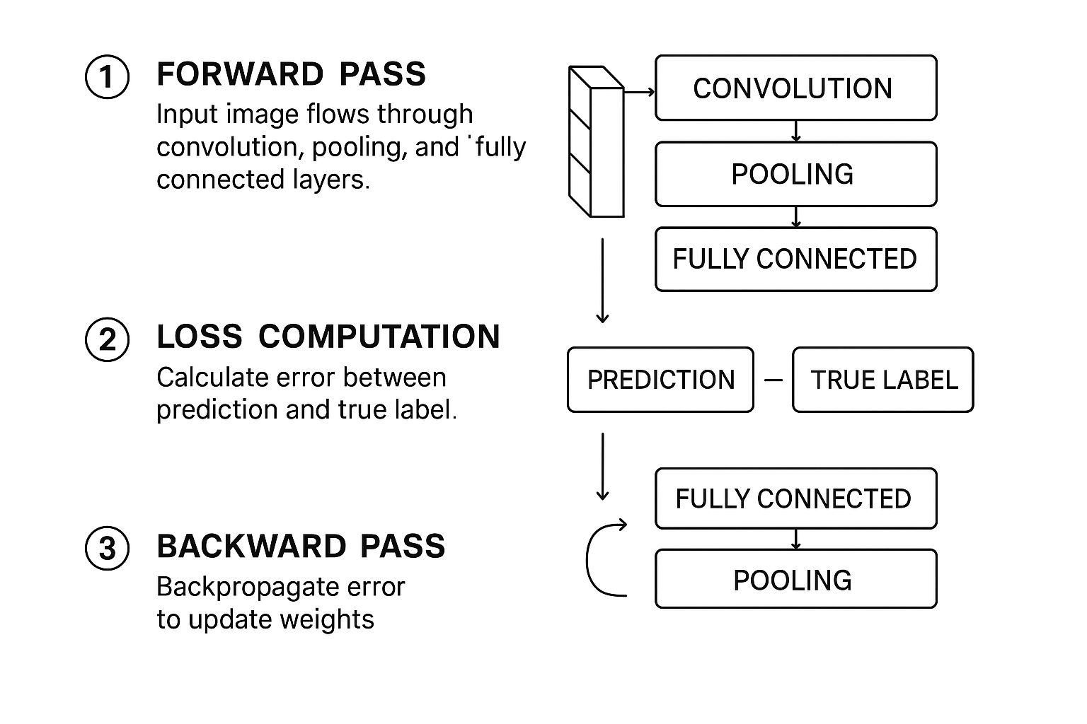
As you can see, it's a continuous feedback loop. The network makes a prediction, measures its error, and then uses that error to update itself for the next round.
The Backward Pass: Learning from Errors
Backpropagation is the clever algorithm that makes this learning possible. It works by taking that error signal from the end and sending it backward through the network, one layer at a time.
Think of it as someone at the finish line shouting, "You were wrong, and here's by how much!" That message travels backward through the layers. At each layer, the algorithm calculates exactly how much each specific filter weight contributed to the final error.
The filters that were most responsible for the wrong guess get adjusted the most. In our example, any filters that lit up for "dog-like" features will be tweaked to be a little less sensitive. On the flip side, filters that might have hinted at "cat-like" features will be strengthened. This entire adjustment process is managed by an optimizer (common ones are Adam or SGD), which carefully updates the weights to push the loss score down.
This complete cycle—forward pass, loss calculation, backward pass—is repeated for every single image in the training dataset. Each repetition nudges the model in the right direction. After seeing thousands or millions of images (these full passes through the data are called epochs), the network’s filters evolve from random noise detectors into highly specialized feature extractors, perfectly tuned to the objects they were trained to see.
This process is incredibly computationally expensive, but it’s what led to the massive breakthroughs in AI. Back in 2012, a model named AlexNet blew the competition away at the ImageNet challenge by using this very technique. Trained on 1.2 million images, it achieved a top-5 error rate of just 15.3%, crushing the previous record of 26.2%. That event kicked off the deep learning explosion. For more on the history of these powerful models on superannotate.com, you can see how quickly things evolved—while AlexNet had 60 million parameters, by 2015, a model like ResNet-152 had that many in its convolutional layers alone.
Exploring Famous CNN Architectures
While knowing the individual layers of a CNN is essential, the real magic happens in how they’re put together. Over the years, a handful of landmark architectures have completely redefined what’s possible in computer vision. These aren't just historical footnotes; they introduced design patterns and breakthroughs we still rely on today.
Think of these famous models as a "greatest hits" collection for solving vision problems. Getting to know them gives you a mental library of proven blueprints. When you're stuck on a new project, you can ask yourself, "Has a famous architecture already solved a problem like this?" It's all about standing on the shoulders of giants.
LeNet-5: The Original Pioneer
Long before "deep learning" was a buzzword, there was LeNet-5. Developed by the legendary Yann LeCun way back in the 1990s, this network was a true trailblazer. It was built for a very practical job: reading handwritten digits on checks.
By today's standards, its structure seems almost quaint, but it laid out the foundational recipe for nearly every modern CNN. The genius was in its simple, repeatable sequence:
- Input: A small grayscale image of a digit.
- Convolution + Pooling: The first block would find basic features like edges and curves.
- Convolution + Pooling: A second block would then combine those simple features into more complex shapes.
- Fully Connected Layers: Finally, these layers acted like a classic neural network to classify the features and decide which digit (0-9) was in the image.
This elegant Convolution -> Pooling -> Convolution -> Pooling pattern proved that a hierarchical approach—learning simple features first and building up—was the way to go. It became the fundamental blueprint for decades of research.
AlexNet: The Game Changer
For a long time, CNNs were mostly an academic curiosity. That all changed in 2012. A network called AlexNet entered the famous ImageNet Large Scale Visual Recognition Challenge (ILSVRC) and didn't just win; it crushed the competition so decisively that the entire AI world snapped to attention.
AlexNet was basically a much bigger, deeper version of LeNet-5, but it brought a few critical innovations to the table. Most importantly, it was one of the first deep networks designed to be trained on GPUs (Graphics Processing Units). This was a huge practical leap, allowing it to chew through the massive ImageNet dataset in a reasonable time.
It also popularized the ReLU (Rectified Linear Unit) activation function, a simple but effective tweak that helped solve nagging training problems that plagued deeper networks.
AlexNet's victory wasn't just a technical win; it was a cultural one. It was the moment that deep learning, powered by CNNs and GPUs, officially became the undisputed king of computer vision.
VGGNet: The Beauty of Simplicity and Depth
After AlexNet's breakout success, researchers started asking a simple question: what happens if we just go deeper? That's exactly what the VGG (Visual Geometry Group) architecture set out to explore. Its philosophy was radical simplicity.
Instead of messing with lots of different filter sizes and complex connections, VGG used one thing and one thing only: tiny 3x3 convolutional filters, stacked one after another, over and over.
This small decision had a massive impact. It turns out that a stack of two 3x3 filters can see the same area as a single 5x5 filter, but it does so with fewer parameters and more non-linear steps. This makes the model both more efficient and more powerful. VGG models, especially VGG16 and VGG19, showed that you could achieve incredible results just by stacking these small, uniform layers very, very deep.
Practical CNN Use Cases You See Every Day

The theory behind CNNs is fascinating, but their real power snaps into focus when you see them in action. You don't have to be a data scientist to use a CNN—in fact, you probably use them dozens of times a day without even realizing it. They're the invisible engines driving many of the "smart" features in your favorite apps.
From unlocking your phone with your face to slapping a filter on your latest Instagram story, CNNs are doing the heavy lifting. Let's pull back the curtain on a few of these common applications to see how abstract theory becomes tangible, everyday convenience.
Object Detection in Your Photo Library
Ever wonder how your phone’s photo gallery automatically groups pictures of your friends, family, or even your pets? That's a classic case of object detection, a task where CNNs absolutely shine. The goal here isn't just to say "this is a cat" but to pinpoint exactly where the cat is in the photo.
Here's a simplified step-by-step tutorial on how a model like YOLO (You Only Look Once) achieves this:
- Grid System: The image is divided into a grid (e.g., 7x7). Each grid cell is responsible for detecting objects whose center falls inside it.
- Bounding Box Prediction: For each grid cell, the CNN predicts several "bounding boxes" and a confidence score for each box. This score reflects how sure the model is that the box contains an object.
- Class Probability: Simultaneously, for each grid cell, the model predicts the probability of different classes (e.g., 80% cat, 15% dog, 5% car).
- Final Output: The system combines these predictions. It keeps the boxes with high confidence scores and multiplies them by the class probabilities to get a final, confident prediction with a tight box around the object.
This is the very process that lets you search your library for "beach" or "birthday cake" and get instant, spookily accurate results.
Semantic Segmentation for Virtual Backgrounds
If you've ever used a virtual background on a video call, you've seen another powerful CNN application in the wild: semantic segmentation. Unlike object detection, which just draws boxes around things, segmentation is way more precise. Its goal is to classify every single pixel in an image.
Here's a step-by-step guide to how it powers that virtual background:
- Pixel-Level Analysis: A specialized CNN (like a U-Net) analyzes the video frame. Instead of outputting a single label, it outputs a "mask" the same size as the original image.
- Create a Mask: In this mask, every pixel is assigned a category. For example, all pixels that are part of a person are labeled '1', and all background pixels are labeled '0'.
- Apply the Mask: The video conferencing software then uses this mask as a stencil. It keeps all the pixels labeled '1' (you) and replaces all the pixels labeled '0' with the virtual background image.
- Repeat for Every Frame: This happens in real-time for every frame of the video, creating the seamless effect of you being somewhere else.
This pixel-level understanding is a huge leap from basic classification. It’s what makes clean cutouts for virtual backgrounds and portrait mode effects possible, and it’s even used in advanced medical imaging where doctors need to isolate specific tissues or organs.
Style Transfer Turning Photos into Art
One of the most visually stunning uses for CNNs is style transfer. This technique takes two images—a "content" image (like your selfie) and a "style" image (like a Van Gogh painting)—and mashes them together. The result? A photo that has the artistic style of the painting applied to the content of your picture.
Here's a simplified tutorial on how an app might do this:
- Feature Extraction: A pre-trained CNN (like VGG19) processes both your photo (content) and the artwork (style). It doesn't try to classify them; it just extracts the feature maps from various layers.
- Separate Content and Style: The algorithm defines "content" as the features from the deeper layers of the network (which see shapes and objects) and "style" as the features from the earlier layers (which see textures and colors).
- Generate a New Image: It starts with a blank, noisy image and iteratively changes it to minimize two types of "loss" or error:
- Content Loss: How different its deep-layer features are from your photo's.
- Style Loss: How different its early-layer features are from the artwork's.
- Find the Balance: The algorithm adjusts the new image until it finds a sweet spot where it looks like your photo but is "painted" with the textures and colors of the artwork.
For a more detailed look, you can learn more about how AI image style transfer works in our dedicated guide.
These examples are just the tip of the iceberg, of course. To get a sense of the sheer scale of AI's impact, which often involves CNNs, it's worth exploring the broader AI industry applications that are changing how businesses operate.
A Few Common Questions About CNNs
As you start working more with convolutional neural networks, a few questions almost always come up. Let's tackle some of the most common ones to help clear up any confusion and solidify your understanding.
We'll cover the fundamental differences between CNNs and other networks, a powerful shortcut called transfer learning, and what kind of hardware you actually need to get started.
How Are CNNs Different from Regular Neural Networks?
The biggest difference comes down to how they "see" the data, especially when it comes to images. A standard neural network, sometimes called a multilayer perceptron, basically flattens an image into one long list of numbers. If you feed it a 100x100 pixel image, it just sees a vector of 10,000 pixel values, completely losing the spatial relationship between them. It has no idea that a pixel at the top left is next to the one beside it.
A CNN, however, is built specifically to understand that structure. Its convolutional layers use filters to scan over the image in small, local patches, preserving the information about how pixels are arranged. This design makes CNNs incredibly good at spotting patterns like edges, textures, and shapes, which is exactly why they're the go-to for just about any computer vision task.
What Is Transfer Learning and Why Is It So Powerful?
Transfer learning is a game-changing technique where you take a model that has already been trained on a massive dataset (like ImageNet, which contains millions of images) and you adapt it for your own, more specific task. Instead of building and training a network from scratch—a process that demands enormous amounts of data and computing power—you start with a model that already knows how to recognize a vast array of visual features.
Here is a practical step-by-step guide to using transfer learning for a custom image classifier (e.g., classifying flower types):
- Choose a Pre-trained Model: Select a well-known architecture like VGG16 or ResNet50, which has already been trained on the ImageNet dataset.
- "Freeze" the Convolutional Layers: Load the model but lock the weights of all the early convolutional layers. These layers have already learned to detect universal features like edges, textures, and shapes, and you don't want to change that.
- Replace the Final Layer: Remove the original final classification layer (which was trained to identify 1000 ImageNet classes) and replace it with a new one tailored to your specific task (e.g., with 5 output neurons for 5 types of flowers).
- Train Only the New Layer: Feed your smaller dataset of flower images to the model. Because most of the network is frozen, you only train the weights of the new final layer. This is much faster and requires far less data.
You can think of transfer learning as standing on the shoulders of giants. You're borrowing the "visual knowledge" a massive model has already learned and just tweaking it for your own project, which can dramatically speed things up.
What Hardware Do I Need to Train a CNN?
Technically, you can train a small CNN on a regular CPU, but you'll find it painfully slow. For any serious deep learning project, a powerful Graphics Processing Unit (GPU) is pretty much a must-have. GPUs are designed to handle thousands of parallel calculations at once, which is exactly the kind of math a CNN relies on. A good GPU can make your training run anywhere from 10 to 100 times faster than a CPU.
If you're just starting out, a modern consumer-grade NVIDIA GPU (like one from their RTX series) will get you far. For bigger, more complex models or commercial-grade work, you'd look at either specialized data center GPUs or cloud computing platforms like AWS, Google Cloud, or Azure. These services let you rent powerful hardware on-demand, so you don't have to deal with the upfront cost.
As you explore more advanced applications, it helps to understand the latest trends. You can get a solid overview by reading our post on what is generative AI.
Ready to put the power of AI to work on your own images? With AI Photo HQ, you can generate stunning, high-quality photos, restore old pictures, and create unique art in seconds. Explore our intuitive platform and see what you can create today at https://aiphotohq.com.


